You’re running along a track. It’s been a while now. You’re sore but you’re forcing yourself to keep going. Your legs are filling with lactic acid. The sun is bearing down on you. It’s hot. It’s grueling.
But you need to know…what will happen if you push yourself to the absolute limit.
Will you make it?
Running a business presents its own similar challenges. You don’t quite know what will happen and there are generally too many variables to predict accurately. You can’t just ‘run harder’ and see how far the business will go. There are market forces outside of your control.
What if you could at least get an idea of the possibilities?
What if you knew the potential range of those variables affecting your business?
You could formulate strategies to hedge your bets. To protect and grow your business in spite of the other factors at work.
This is where Monte Carlo simulation comes into play.
This technique isn’t all that new but it’s still used extensively in fields where there is risk involved. Breaking it down really simply, Monte Carlo simulation allows you to guesstimate the range (read: best case and worst case) of values that a variable might take. This might mean predicting the range of values for a particular commodity (which might feed into a revenue model) or the value of a particular financial instrument (which might feed into a capital adequacy framework).
It’s extremely useful as an input into scenario-based forecasts. What’s even better? You can do it pretty easily using free external data sources and TM1. Give it a go below! Hit the green button to download the example codebook and follow along.
1. Get Data Using Pandas DataReader
There are a whole heap of free resources that you can use to get free data for your project. One of the best and probably one of the easiest to use is Pandas DataReader. With a few lines of code, you’re able to access data from Yahoo Finance, Google, FRED, World Bank etc. The list goes on.
Given how much petrol prices tend to range each week I figured crude oil prices would probably be a good candidate for this demo. A quick search on Quandl provided a number of crude oil data sources.
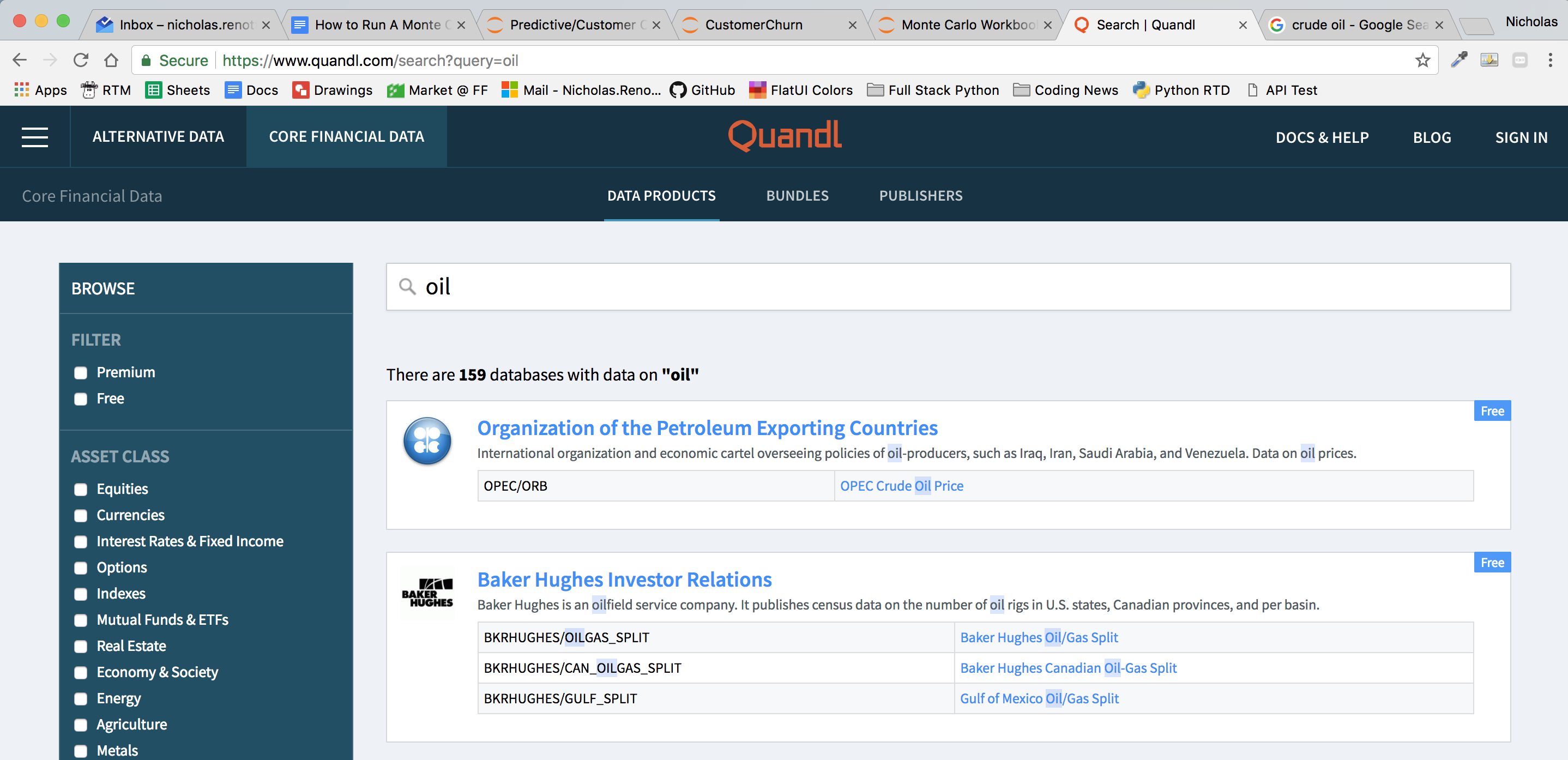
There are 4 parameters that need to be passed to the DataReader function to get the right dataset. These are the instrument, the data source and the start and end date. The instrument is OPEC/ORB (OPEC Crude Oil Basket Price) and the date range is 3 Jan 2017 to 31 Dec 2017.
First, import the required modules.
# Import data reader
import pandas_datareader.data as web
# Import pandas
import pandas as pd
# Import datetime for date manipulation
import datetime as dt
Then format the date range appropriately using DateTime.
# Set start and end datetime for web pull
year = 2017
start = dt.datetime(year,1,3)
end = dt.datetime(year,12,31)
Then run the query.
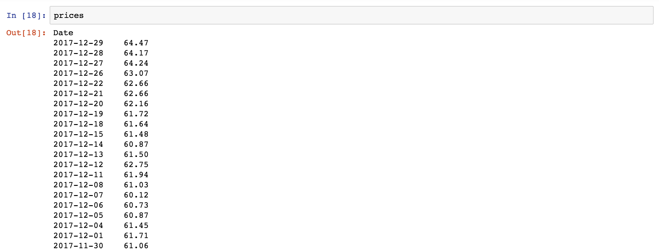
# Get price data from quandl using pandas web reader
instrument = "OPEC/ORB"
prices = web.DataReader(instrument, "quandl", start, end)['Value']
The prices data series should look a little like this.
2. Run the simulation
This Monte Carlo simulation uses the daily volatility (aka the standard deviation of returns) to forecast the range of possible oil prices in the future. It does this by applying a random “growth” factor to the previously forecasted value. This growth factor is a random number between 0 and the calculated daily volatility.
Why does this work? Well, once we have a pretty good idea of the daily volatility we can apply a random growth factor that is capped at the daily volatility of our simulation. By doing the same thing over and over we can get a pretty good idea of the range that the price is going to be over the simulation period.
There are a few things that need to be calculated before running the simulation these are the daily return and the daily volatility. You’ll also need to import numpy for this next step to generate random numbers for the simulation.
# Import numpy for math functions/random
import numpy as np
# Get percent change pd function from price array
returns = prices.pct_change()
# Calculate daily volatility for random walk
daily_vol = returns.std()
# Get the last price
last_price = prices[-1]
Then set up the number of trials/simulations we want to run plus the number of days in the trial.
# Set number of trials for simulation
trials = 1000
# Set number of days within dataset
days = 240
As well as a placeholder dataframe to store the results.
# Create placeholder dataframe to store results
simulation_df = pd.DataFrame()
Finally, run the simulation.
# Loop through trials
for trial in range(trials):
# Set day to zero
day = 0
# Create placeholder array for simulation
price_series = []
# Get random value between 0 and daily volatility
rand = (1+ np.random.normal(0, daily_vol))
# Apply volatility to last price
price = last_price * rand
# Add value to random walk series
price_series.append(price)
# Loop through days
for day in range(days):
if day == 240:
break
# Get price from previous day and apply daily volatility
price = price_series[day] * (1+np.random.normal(0, daily_vol))
# Add to random walk series
price_series.append(price)
# Increment day counter
day += 1
# Add random walk series to simulation dataframe
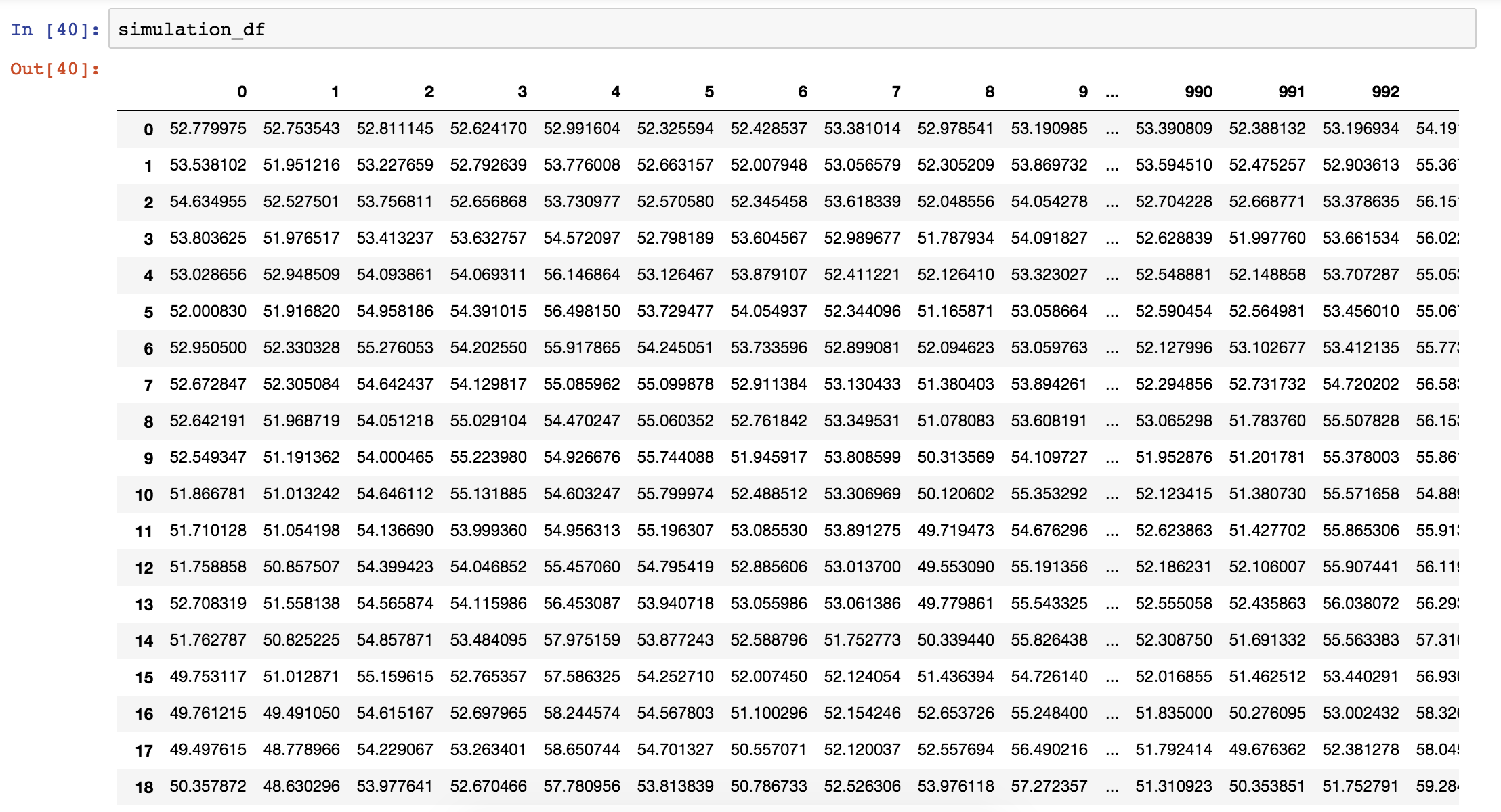
simulation_df[trial] = price_series
The results are stored in the simulation_df dataframe. Each column represents a separate trial and each row is a separate day within each simulation.
3. Plot and Analyse the Results
We can analyse the results of the simulation by plotting out what’s just happened. Matplotlib makes it relatively easy to plot each simulation.
Import pyplot.
# Import pyplot for plotting
import matplotlib.pyplot as plt
%matplotlib inline
The setup and display the plot.
# Create plot area
fig = plt.figure()
# Set the title
fig.suptitle('Monte Carlo Simulation:OPEC/ORB')
# Set the plot data
plt.plot(simulation_df)
# Set a fixed line displaying the last price
plt.axhline(y=last_price, color = 'r', linestyle = "-")
# Set x label
plt.xlabel('Day')
# Set y label
plt.ylabel('Price')
# Show the plot
plt.show()
You should get something that looks a little like the graph below. Don’t fret if the plot isn’t exactly the same as the simulation is using a different set of random numbers each time.

You can also get some summary stats by using the pandas describe method.
simulation_df.tail(1).transpose().describe()
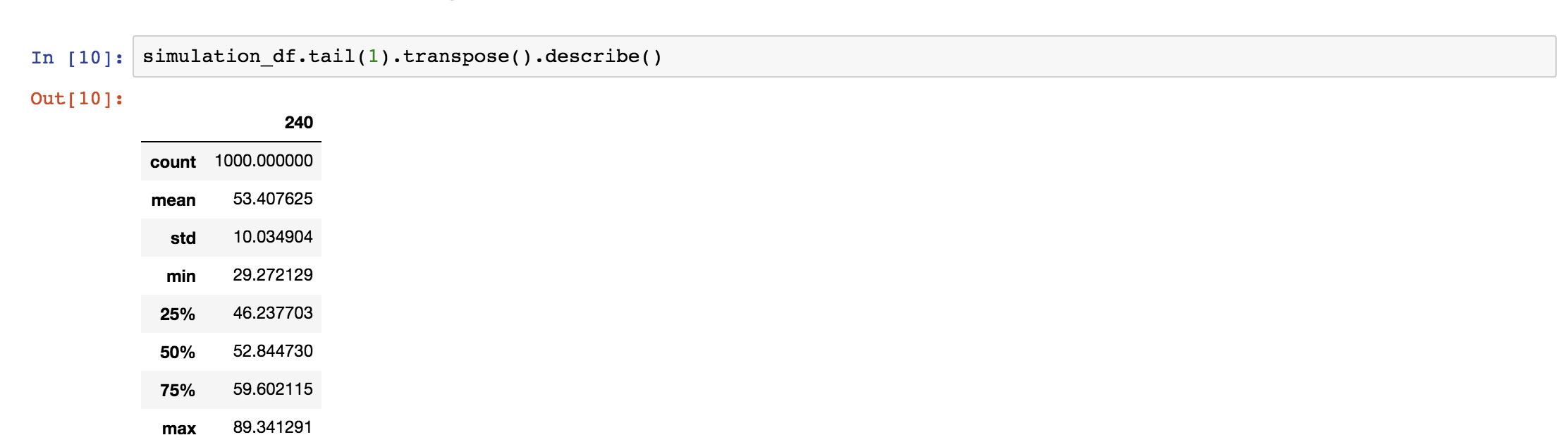
This is particularly useful if you’re analysing the final expected range of values (aka day 240 in this case). You can get a pretty good idea of the range of values you might want to plug into a stress test or cost forecasting model.
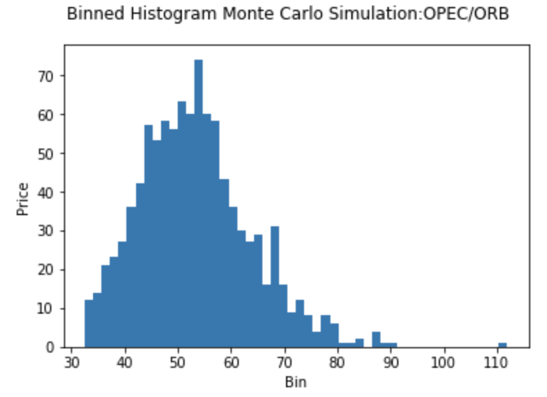
We can also plot the expected range of values in separate bins.
# Final day of the simulation
final = simulation_df.tail(1)
# Show binned histogram of simulation
plt.hist(final, bins = 50)
plt.suptitle('Binned Histogram Monte Carlo Simulation:OPEC/ORB')
# Set x label
plt.xlabel('Bin')
# Set y label
plt.ylabel('Price')
plt.show()
4. Send Results Into TM1
Last but not least we can send these results into TM1 where they can be plugged into another model (stay tuned: I’ll be building a full blown financial model using this in the next month!).
First, transpose and transform our data set into a cellset (aka a python dict).
result = simulation_df.transpose()
data = {}
for trial in result.index:
    for day in result.columns:
        data[(instrument,year,day+1,trial+1,"Value")] = result.iloc[trial,day]
Then import TM1py.
# Import TM1 Service module
from TM1py.Services import TM1Service
# Import TM1 utils module
from TM1py.Utils import Utils
# MDX view
from TM1py.Objects import MDXView
Set your TM1 config parameters.
# Set TM1 config parameters
address = "localhost"
port = 45678
user = "admin"
password = ""
ssl = True
And send it back into TM1.
# Import time module for timing
import time
# Calculate number of datapoints
cells = len(data)
# Calculate start time
start = time.time()
# Create new instance of TM1 Service object and load data
with TM1Service(address= address, port=port, user=user, password=password, ssl=ssl) as tm1:
   tm1.cubes.cells.write_values('Monte Carlo', data)
# Calculate end time
end = time.time()
# Calculate time elapsed
timeelapsed = end-start
# Calculate write speed cells divided by time elapsed
writespeed =  cells/timeelapsed
# Print result
print('Data loaded to cube. Time elapsed {0} seconds. Write speed is {1} cells per second.'.format(timeelapsed,writespeed))
And that’s it, your simulation is now stored safely in TM1.

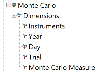
For reference, these were the dimensions in the cube that was used for this model.
This technique has a whole range of applications. Imagine plugging it directly into your forecast, you would be able to get a better range of possible estimates in the blink of an eye. What are you waiting for! Spin up a TM1 instance and install TM1py and give it go!
Other Resources