It hits you a freight train. You never ever saw it coming. You keep hearing the words over and over again in your head…
“We lost our biggest account.”
The reality starts to sink in. You start thinking of ways to fix it.
“How can we get them back?”
“What went wrong?”
“Why me?”
Deep down you know that it’s probably a lost cause. If only you could’ve seen this coming. Maybe. Just maybe, you could have done something to keep them on. Maybe offering dedicated support. Cutting them a better deal. Or just giving them some more face time. You know you could have done something if you had known early on. But you didn’t, at least not early enough.
But what if you could know earlier? What if you had a better idea of whether or not a customer was likely to leave or not?
You could implement retention strategies.
Reduce new lead marketing costs.
Keep customers happy.
And ultimately, improve the bottom line.
Well, you can.
The tutorial below goes through how to use TM1py and Scikit Learn to predict Customer Churn(AKA the chance of customers leaving or not repurchasing) and how to automatically send it back into TM1. The data used is based off the publicly available Telco Customer Churn dataset which can be found here. However, this could just as easily be extended to tap into Salesforce or your existing customer database.
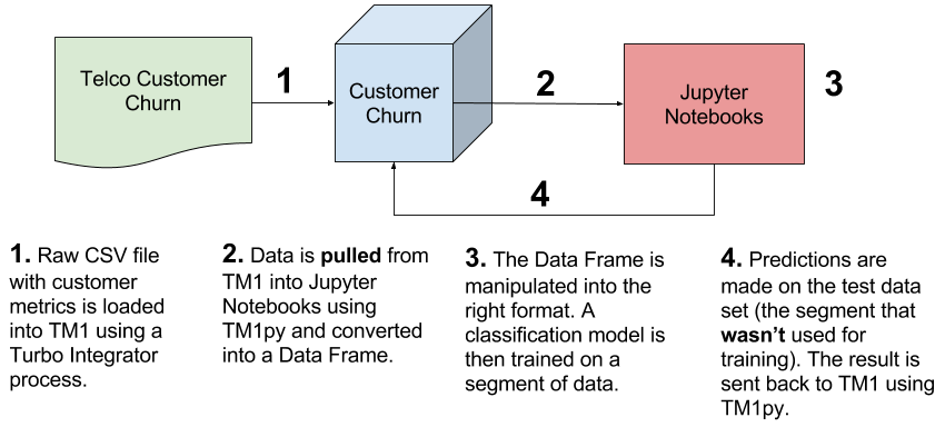
How it works
At a super-high level, this is how it all fits together. Data is loaded into TM1 using a TI process. A view is pulled into Jupyter Notebooks using TM1py. The data is then reformatted and a model is trained. Finally, predictions are made and the result is sent back into TM1. The diagram below sums this all up.
Step 1: Import the required modules
Before stepping through the process there are a number of modules that need to be imported. This model relies heavily on Pandas for data manipulation and transformation and TM1py for interacting with the TM1 API. Later on, Scikit learn is imported to deal with model training and prediction.
# Import tm1 service module
from TM1py.Services import TM1Service
# Import tm1 utils module
from TM1py.Utils import Utils
# MDX view
from TM1py.Objects import MDXView
# Import pandas
import pandas as pd
# Import matplotlib
import matplotlib.pyplot as plt
# Inline plotting for matplotlib
get_ipython().magic('matplotlib inline')
# Import seaborn
import seaborn as sns
# Import numpy
import numpy as np
Step 2: Load TM1 parameters
Consistently setting parameters in a Jupyter Notebook can become a little repetitive, especially if you’re always connecting to the same TM1 model. Rather than declaring these details in the code, you can change your parameters in a JSON config file and load them once using the code below. This allows global config parameters to be set once rather than retrieving them each time a new notebook is created. To do this simply open config.json and update the following parameters with your TM1 details:
       "adminhost":"localhost",
       "HTTPPort": "8882",
       "username":"admin",
       "password":"",
       "ssl":"True"
# Import json package
import json

# Import config file data
with open('config.json') as json_data_file:
    cfg = json.load(json_data_file)

# Set all tm1 parameters
address = cfg[0]['adminhost']
port = cfg[0]['HTTPPort']
user = cfg[0]['username']
password = cfg[0]['password']
ssl = cfg[0]['ssl']
To make selecting your cube and view a little easier, the Ipython widgets have been used to create drop-down selectors. This sort of makes the model a little more end-user friendly.
cubes = []

with TM1Service(address= address, port=port, user=user, password=password, ssl=ssl) as tm1:
    dim = '}Cubes'

     Get control cubes dimension to get a list of all cubes
    dimension = tm1.dimensions.get(dim)

     Get the hierarchy from the dimension
    for hierarchy in dimension:
         Loop through each element and attach it to the list
        for element in hierarchy:
            cubes.append(element.name)
# Import py widgets for dropdown selector
import ipywidgets as widgets

# Set selector value = to cube
cube = widgets.Dropdown(
options=cubes,
value='General Ledger',
description='Cube:',
disabled=False,
)

# Display dropdown
cube

views = []
#HUGE thanks to Marius Wirtz for helping me out with this!
with TM1Service(address= address, port=port, user=user, password=password, ssl=ssl) as tm1:

    cube_name = str(cube.value)

    # Get all private and public views
    private_views, public_views = tm1.cubes.views.get_all(cube_name=cube_name)

    # Create a list of views
    for view in public_views:
        views.append(view.name)
# Create ipython dropdown widget to store view value
view = widgets.Dropdown(
    options=views,
    value=views[0],
    description='View:',
    disabled=False,
)

# Output view dropdown
view

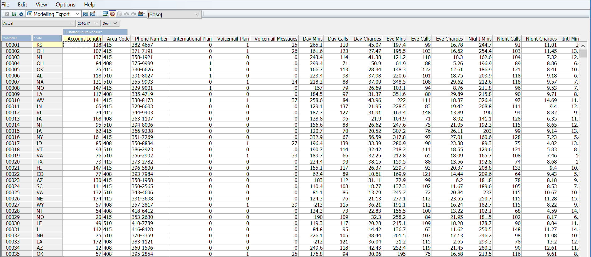
The modeling view looks a little like the view below. This is a direct load of the telco customer churn data set loaded to numbered customers and some other placeholder variables (e.g. Version, Year, Month etc).
Step 3: Get TM1 Data and reformat the DataFrame
Next, you’ll need to get your data from TM1. This is almost identical to the code used for the Time Series Forecasting. The code connects to TM1 and grabs the data set shown above. The result is converted into a (multi-indexed) pandas DataFrame.
For more on Pandas and DataFrames check out this pandas tutorial.
It’s important to note that before importing any data, the view needs to have already been created. All you’re doing here is retrieving the view and reshaping the DataFrame so that it’s easy to work with for modeling.
# With block to connect to TM1 resource, the config params are stored in the cfg.JSON file
with TM1Service(address= address, port=port, user=user, password=password, ssl=ssl) as tm1:
    # Specify cube view that you want to analyse
    # This draws from the dropdowns above but can be overwritten here
    cube_name = str(cube.value)
    view_name = str(view.value)

    # Extract MDX from CubeView
    mdx = tm1.cubes.views.get_native_view(cube_name, view_name, private=False).MDX
    print(mdx)

    # Get data from P&L cube through MDX
    rawdata = tm1.cubes.cells.execute_mdx(mdx)

    # Build pandas DataFrame fram raw cellset data
    df = Utils.build_pandas_dataframe_from_cellset(rawdata)
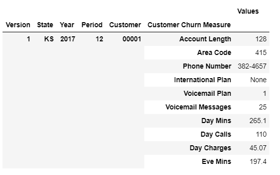
# Remove the multi index
df = df.reset_index()

# Create a new index and set
idx = ['Version','State', 'Year', 'Period', 'Customer', 'Customer Churn Measure']
df = df.set_index(idx)

# Unstack the DataFrame
df = df.unstack(5)
df = df.reset_index()

# Bring TM1 Measures to the same level as dimensions
# Dimensions are stored at level 0
lv0 = df.columns.get_level_values(0)

# Measures are stored at level 1 (in this instance)
lv1 = df.columns.get_level_values(1)

# Collate the columns
columns = lv0[:5]
columns = columns.append(lv1[5:])

# Reset the column values
df.columns = columns

# Check out the reformatted DataFrame
df.head()
The dataframe will go from looking like this…
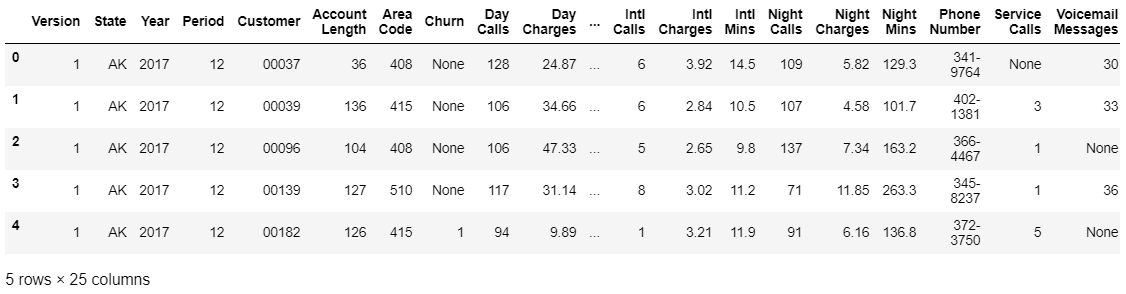
To this…
Step 4: Exploratory Analysis and Data Prep
It’s always a good idea to get an understanding of what your data looks like. In practice, this is called exploratory analysis and should be relatively brief. This would typically fall under the Data Understanding section of the Cross Industry Standard Process for Data Mining (CRISP-DM).
At the same time, it’s important to get the best quality data possible. Why? Because better data beats fancy algorithms every time! In this case, both exploratory analysis and data cleaning are included in the section below.
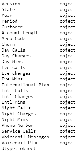
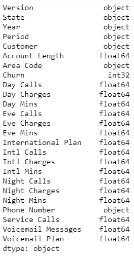
# Review column datatypes
df.dtypes
Running df.dtypes returns the data types for each of the features/columns within the data frame. The object data type is native to the Pandas package, think of it as string data. Before going ahead and actually trying to predict anything the features (variables used to predict) need to be converted into the right data types. In this case, converting string data to floats or integers.
# Feature columns that should be converted to floats
floats = df.drop(['Version','State','Year','Period','Customer','Phone Number','Area Code', 'Churn'], axis=1 ).columns

# Convert and fill blanks
df[floats] = df[floats].fillna(0).astype(float)

# Convert Churn measure to an integer (1,0)
df["Churn"] = df["Churn"].fillna(0).astype(int)
# Check data types have updated
df.dtypes
The new data types…we have floats!
When you’re training a new model you typically need to be selective with the features that you choose to train the model on. This process is known as feature selection (go figure right?). There are a number of different ways to do this but the end goal is to choose the “best” number of features that yields the best possible accuracy whilst at the same time preventing overfitting. You can read more about feature selection here.
In this case, the Version, State, Year, Period and Customer aren’t variables that are needed but are useful for referencing each row of data. By setting these variables as an Index, they’re still available for referencing but won’t be included when the model is trained.
# Create a list of index columns
index = ['Version','State', 'Year', 'Period', 'Customer']

# Set the index
df = df.set_index(index)
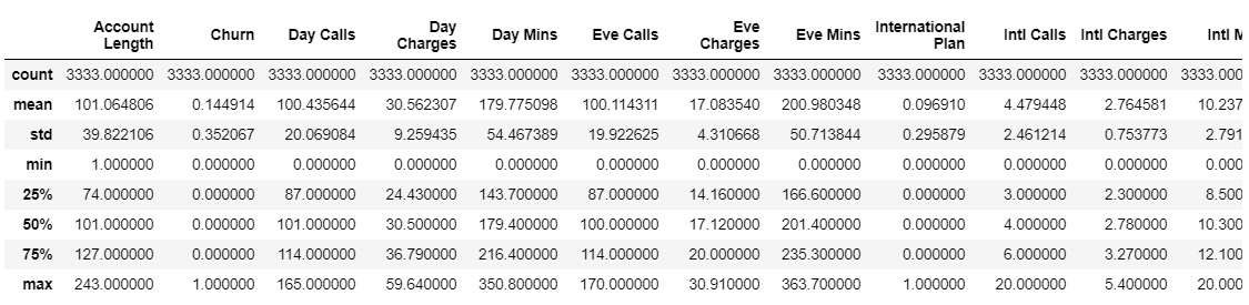
It’s always a good idea to get a good handle on the data that you’re using. Running df.describe, plotting the feature variables and creating segmentation helps to get an idea of trends and anomalies in your data.
# Review summary statistics for continuous features
df.describe()
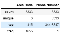
# Summary stats for non-continuous features
df.describe(include=['object'])
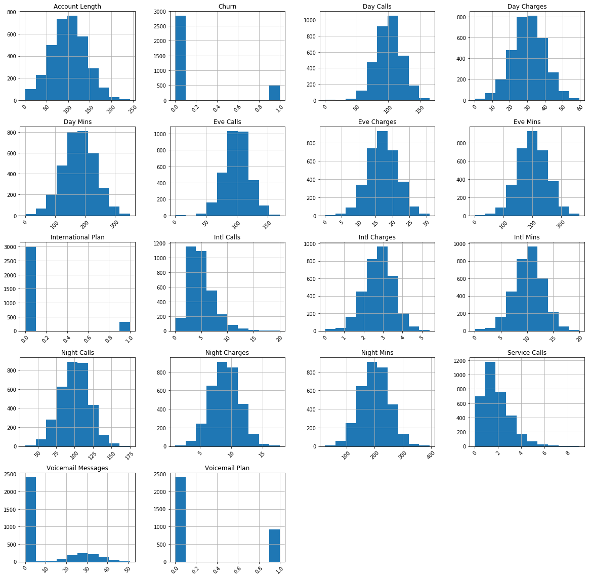
# Visualise each continuous feature
df.hist(figsize=(20,20),xrot = 45)
plt.show()
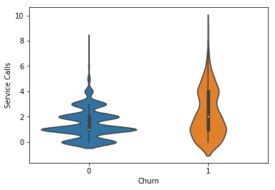
# Create violin plot to segment Service Calls
sns.violinplot(y="Service Calls", x="Churn", data=df)
plt.show()
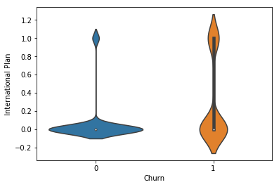
# Create violin plot to segment International Calls
sns.violinplot(y='International Plan', x='Churn', data=df)
plt.show()
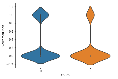
# Create violin plot to segment customers with a Voicemail Plan
sns.violinplot(y='Voicemail Plan', x='Churn', data=df)
plt.show()
Step 5: Train the model
This model determines the likelihood of customer churn by classifying them into one of two classes (likely to churn or not likely to churn). This is accomplished by splitting the DataFrame into a Training DataFrame and Testing DataFrame. The model is ‘trained’ on the training data by tuning/choosing parameters that attempt minimise the chance of predicting incorrectly. The trained model is then applied (Step 6) on the testing dataframe (which the model has never seen before) to make churn predictions.
# Import sklearn
import sklearn

# Import Logistic Regression
from sklearn.linear_model import LogisticRegression

# Import RandomForestClassifier and GradientBoostingClassifer
from sklearn.ensemble import RandomForestClassifier, GradientBoostingClassifier

# Function for splitting training and test set
from sklearn.model_selection import train_test_split  Scikit-Learn 0.18+

# Function for creating model pipelines
from sklearn.pipeline import make_pipeline

# For standardization
from sklearn.preprocessing import StandardScaler

# Helper for cross-validation
from sklearn.model_selection import GridSearchCV

# Classification metrics (added later)
from sklearn.metrics import roc_curve, auc
Before training your model you need to split your dataset into training and testing data. This way, you’re able to train your model on a data set and test how well it predicts on a completely different set of data. The following code block takes care of splitting the existing dataframe.
# Set X - feature set and y - the target variable in this case Churn
y = df['Churn']
X = df.drop(['Area Code','Phone Number','Churn'], axis = 1)

# Create train and test data splits
X_train, X_test, y_train, y_test = train_test_split(X, y,
                                                    test_size=0.2,
                                                    random_state=1234,
                                                    stratify=df['Churn'])
The large majority of the code below has been retrofitted from the Elite Data Science Machine Learning Master Class to integrate with data from TM1. I highly recommend you check out the course if you’re interested in learning more about machine learning in Python!
# Create pipeline
pipelines = {
    'l1' : make_pipeline(StandardScaler(),
                         LogisticRegression(penalty='l1' , random_state=123)),
    'l2' : make_pipeline(StandardScaler(),
                         LogisticRegression(penalty='l2' , random_state=123)),
    'rf' : make_pipeline(StandardScaler(), RandomForestClassifier(random_state=123)),
    'gb' : make_pipeline(StandardScaler(), GradientBoostingClassifier(random_state=123))
}

# Setup hyper parameter ranges
# l1 logistic regression hyperparams
l1_hyperparameters = {
    'logisticregression__C' : np.linspace(1e-3, 1e3, 10),
}
# l2 logistic regression hyperparams
l2_hyperparameters = {
    'logisticregression__C' : np.linspace(1e-3, 1e3, 10),
}
# Random Forest hyperparams
rf_hyperparameters = {
    'randomforestclassifier__n_estimators': [100, 200],
    'randomforestclassifier__max_features': ['auto', 'sqrt', 0.33]
}
# Gradient Boosted hyperparams
gb_hyperparameters = {
    'gradientboostingclassifier__n_estimators': [100, 200],
    'gradientboostingclassifier__learning_rate': [0.05, 0.1, 0.2],
    'gradientboostingclassifier__max_depth': [1, 3, 5]
}

# Create hyperparameters dictionary
hyperparameters = {
    'l1' : l1_hyperparameters,
    'l2' : l2_hyperparameters,
    'rf' : rf_hyperparameters,
    'gb' : gb_hyperparameters
}
This next step actually begins to train the model over four different machine learning algorithms. These are L1 and L2 logistic regression, Random Forests and Gradient Boosting. This can take between 5-20 minutes depending on your machine. Sit back and enjoy a cuppa whilst this is running.
# Create empty dictionary called fitted_models
fitted_models = {}

# Loop through model pipelines, tuning each one and saving it to fitted_models
for name, pipeline in pipelines.items():
    # Create cross-validation object from pipeline and hyperparameters
    model = GridSearchCV(pipeline, hyperparameters[name], cv=10, n_jobs=-1)

    # Fit model on X_train, y_train
    model.fit(X_train, y_train)

    # Store model in fitted_models[name]
    fitted_models[name] = model

    # Print '{name} has been fitted'
    print(name, 'has been fitted.')

# Display best_score_ for each fitted model
for name, model in fitted_models.items():
    print( name, model.best_score_ )

# Import classification metrics
from sklearn.metrics import roc_curve, auc

# Predict classes using Random Forest
pred = fitted_models['rf'].predict(X_test)
# Display first 5 predictions
pred[:5]

# Import confusion_matrix
from sklearn.metrics import confusion_matrix

# Display confusion matrix for y_test and pred
print( confusion_matrix(y_test, pred) )

# Predict PROBABILITIES using Random Forest Ensemble
pred = fitted_models['rf'].predict_proba(X_test)

# Get just the prediction for the positive class (1)
pred = [p[1] for p in pred]

# Display first 5 predictions
pred[:10]
# Calculate ROC curve from y_test and pred
fpr, tpr, thresholds = roc_curve(y_test, pred)
# Store fpr, tpr, thresholds in DataFrame and display last 10
pd.DataFrame({'FPR': fpr, 'TPR' : tpr, 'Thresholds' : thresholds}).tail(10)
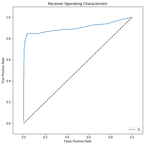
# Initialize figure
fig = plt.figure(figsize=(8,8))
plt.title('Receiver Operating Characteristic')
# Plot ROC curve
plt.plot(fpr, tpr, label='l1')
plt.legend(loc='lower right')
# Diagonal 45 degree line
plt.plot([0,1],[0,1],'k--')
# Axes limits and labels
plt.xlim([-0.1,1.1])
plt.ylim([-0.1,1.1])
plt.ylabel('True Positive Rate')
plt.xlabel('False Positive Rate')
plt.show()
The Receiver Operating Curve (ROC) curve tells you how well your model performed. As a general rule, the blue line should follow the right axis and top axis as closely as possible.
Pickle allows you to save your trained model for use later on. This means that rather than re-training your model each and every time you want to predict churn you can pick up where you left off. Step 6 picks up from this point. If you’ve already trained your model once before and saved a Pickle file, you can skip to Step 6!
# Import pickle
import pickle
# Save the best model
with open('final_model.pkl', 'wb') as f:
    pickle.dump(fitted_models['rf'].best_estimator_, f)
Step 6: Predict Customer Churn
Now that your model is trained…you can use it to predict stuff! The next set of code blocks uses the pre-trained model to predict churn on the feature variables. Once you’ve completed the training steps above (which takes around 5-10 minutes) you can continue using the same Pickle output file below to predict without having to frequently retrain your model. It is, however, a good idea to retrain your model periodically or once you start to see accuracy decrease.
# Open the trained model
with open('final_model.pkl', 'rb') as f:
    model = pickle.load(f)

# Set target variable
y = df['Churn']

# Set feature columns
X = df.drop(['Area Code','Phone Number','Churn'], axis = 1)

#Create a new train/test split
X_train , X_test , y_train , y_test = train_test_split(X, y,
    test_size=0.2,
    random_state=1234,
    stratify=df['Churn'])

# Predict the train values (little redundant but we'll send these back into TM1)
predtrain = model.predict_proba(X_train)

# Predict the testing data
predtest = model.predict_proba(X_test)

# Store the training predictions
predtrain = [p[1] for p in predtrain]

# Store the test predictions
predtest = [p[1] for p in predtest]
Step 7: Send it back into TM1
Finally, send the data back into TM1!
# Collate the X values (features) and predictions for the train data
trainres = X_train
trainres['Churn'] = y_train
trainres['Prediction'] = predtrain

# Collate the X values (features) and predictions for the testing data
testres = X_test
testres['Churn'] = y_test
testres['Prediction'] = predtest

# Consolidate the results into a flat DataFrame
result = trainres
result = result.append(testres)
result = result.reset_index()

## Ignore the warning ##
with TM1Service(address= address, port=port, user=user, password=password, ssl=ssl) as tm1:

    # Cellset to store the new data
    cellset = {}

    # Populate cellset with coordinates and value pairs
    for index, row in result.iterrows():

        # Create cellset that maps to the TM1 cube - effective creating a CELLPUT
        cellset[(row['Version'],row['State'],row['Year'], row['Period'], row['Customer'], 'Prediction')] = row['Prediction']

        # Send the values
        tm1.cubes.cells.write_values('Customer Churn', cellset)
The end result is sent back into the same Customer Churn cube under the Prediction measure. The value stored is actually the probability that a customer is likely to churn i.e. it’s a sliding scale. Adding a rule to the Churn Prediction measure allows you to get a binary (1-churn, 0-no churn) value.
SKIPCHECK;
# Rule 1: If customer churn probability is greater than 50% set value to 1
['Churn Prediction'] = N:IF(['Prediction'] < 0.5, 0, 1);
FEEDERS;
# Feeder 1
['Prediction'] => ['Churn Prediction'];
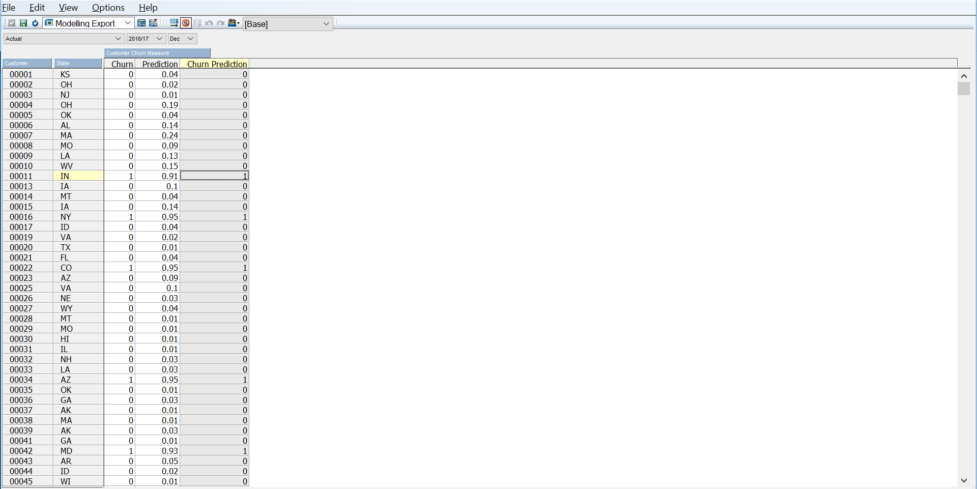
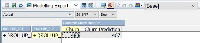
You should now be able to see the original Churn value and the prediction that’s been created side by side when rolled up!
Want to implement this in your business? Download the free source code below…