You’re stumped. You thought you had it all worked out. You were so close. But nope. At the meeting someone had thrown a spanner into the works and POOF you’re perfect schedule was shot. You’d just spent 13 days trying to create a production schedule. Now you’re going to have to start all over again. All because of a slight change in demand levels and machine up time.
*DING*
Why didn’t you think of this earlier? EXCEL SOLVER! Hold it right there.
Before you spend countless hours trying to get Excel solver to work let me introduce you to a better solution…da da da DAAA.
Solver for TM1!
Solver is really just a graphical user interface that allows you to work out linear programming problems in Excel. You can model ridiculously complex (or super simple) problems just the same in TM1 using PuLP and TM1py. But before you jump ahead…let’s run through some basics. If you’re all over it head on over to Step 1 to get cracking on the walkthrough.
What is Linear Programming?
The best answer I could come up with is the metadata explanation from Analytics Vidhya:
Linear programming is used for obtaining the most optimal solution for a problem with given constraints.
Okay, breaking this down a little more. Imagine you wake up after a huge night out. You’re starving. Your only thought right now is to eat as much as humanly possible. But….after going all out last night you’ve only got $20 left in your wallet. You could spend the $20 and buy a salad and some coconut water or you could go wild and buy two pizzas from Pizza Hut.
Eating as much as humanly possible isn’t exactly a quantifiable goal. Instead, let’s say you want to eat as many calories as possible. Assume the two meals cost the same price i.e. the salad and coconut water is $20 and each pizza is $10 (so you can get two). Each pizza has a caloric value of 2,000 calories and the salad combo has a caloric value of 900 calories. You’re clearly going to get more calories by ordering the two pizzas. As a result, you end up ordering the two pizzas and maximizing your calories (and your happiness) from the $20. This scenario can be represented as a linear programming problem.
The facts:
- Your constraint = $20 you have remaining
- Calories from each pizza = 2,000
- Calories from salad combo = 900
- Price of one pizza = $10
- Price of salad combo = $20
Given the above, the problem function is this:
calories = 2000 * number of pizzas + 900 * number of salad combos
In this case, you’re trying to maximize the number of calories. This is pretty straightforward. You set your number of pizzas AND number of salad combos as high as possible (i.e. infinity) and you’ll get an infinite number of calories.
BUT
Remember that you only have $20 to spend. This is a constraint which limits your ability to buy an infinite number of pizzas and salads. This means that you have to try to maximize the function above whilst taking into account the following constraint:
$20 = $10 * number of pizzas + $20 * number of salad combos
If you solve these equations simultaneously whilst aiming to maximize calories you’ll end up ordering 2 pizzas. (I should probably add that you can’t order negative pizzas or salads.) This is a pretty simple linear programming example but you can pretty quickly see that it can be used for a whole variety of optimization problems.
One super useful application of Linear Programming is optimal scheduling. In this case, determining which factories to use for manufacturing. This tutorial uses Pulp and TM1py to determine these parameters for a manufacturing plant. The majority of the modeling in this tutorial is based on the awesome set of tutorials by Ben Alex Keen. I’ve really just tweaked and tested it a little to get it to fit into a TM1 model!
-
Build and Load TM1 cubes
You can download the two TI processes to create and load the TM1 cubes in the download pack above. Assuming you’ve already done that you can access the data using Jupyter by importing the views using TM1py. First import the modules below.
# Import tm1 service module
from TM1py.Services import TM1Service
# Import tm1 utils module
from TM1py.Utils import Utils
# MDX view
from TM1py.Objects import MDXView
# Import pandas
import pandas as pd
And setup your TM1 config parameters so that you can connect to TM1 using the API. Remember to replace these values with the relevant details for your TM1 application.
# Set TM1 config parameters
address = "localhost"
port = 45678
user = "admin"
password = ""
ssl = True
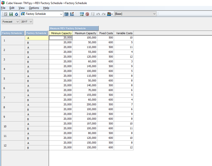
The two views that the model relies on are the Factory Schedule view from the REV Factory Schedule cube
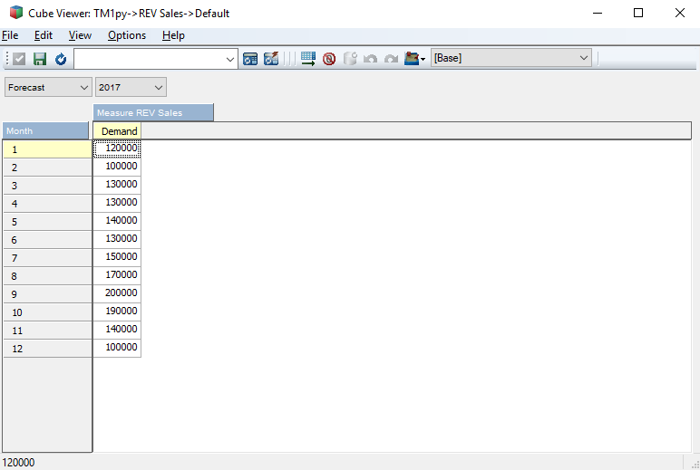
and the Forecast Demand view from the REV Sales cube.
The next block creates a TM1Service object from the TM1py module that allows you to grab data and interact with your TM1 instance using the API. This is the basic recipe to grab data (they’re also the same steps that I’ve used in the majority of the TM1 tutorials).
Create an MDX statement from the view that already exists in TM1.
with TM1Service(address= address, port=port, user=user, password=password, ssl=ssl) as tm1:
    # Get Schedule and Demand data
    sched_cube = 'REV Factory Schedule'
    sched_view = 'Factory Schedule'

    # Extract MDX from CubeView
    sched_mdx = tm1.cubes.views.get_native_view(sched_cube, sched_view, private=False).MDX
Execute the MDX to grab data, this returned dataset is returned as a dictionary by default.
# Get data from P&L cube through MDX
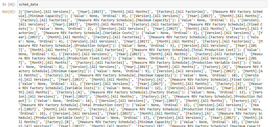
sched_data = tm1.cubes.cells.execute_mdx(sched_mdx)
Rather than working with a dictionary for analysis, the TM1py method build_pandas_dataframe_from_cellset allows you to quickly transform the dictionary into a pandas data frame.
# Build pandas DataFrame fram raw cellset data
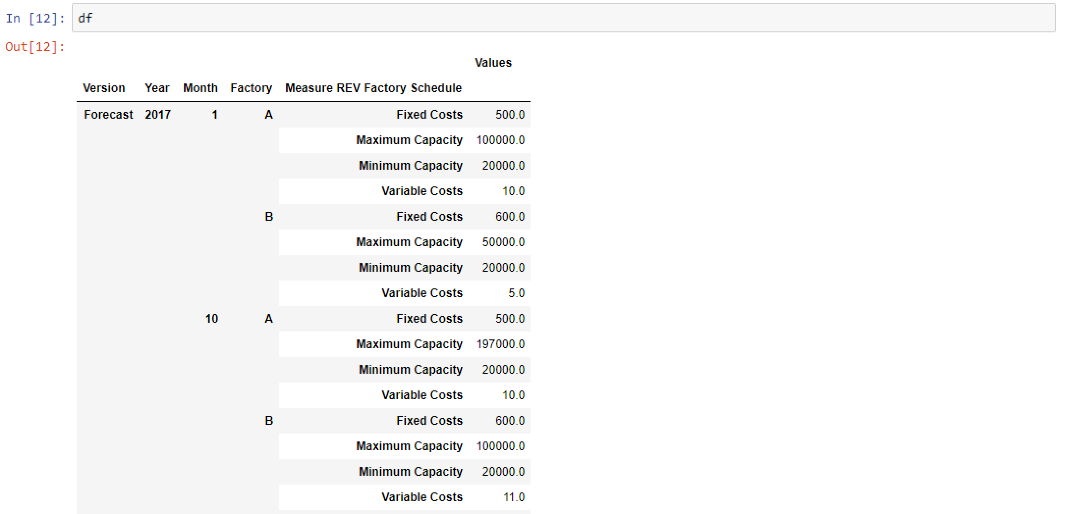
df = Utils.build_pandas_dataframe_from_cellset(sched_data)
It takes data that looks like this…
And transforms it into this…
This entire sequence is repeated for the REV Sales cube in order to pull demand data. This is the full code block for both cubes and view. The exact same sequence (i.e. View, MDX, DataFrame) is repeated just with alternate naming conventions.
with TM1Service(address= address, port=port, user=user, password=password, ssl=ssl) as tm1:

    # Get Schedule and Demand data
    sched_cube = 'REV Factory Schedule'
    sched_view = 'Factory Schedule'

    # Extract MDX from CubeView
    sched_mdx = tm1.cubes.views.get_native_view(sched_cube, sched_view, private=False).MDX

    # Get data from P&L cube through MDX
    sched_data = tm1.cubes.cells.execute_mdx(sched_mdx)

    # Build pandas DataFrame fram raw cellset data
    df = Utils.build_pandas_dataframe_from_cellset(sched_data)

    # Get expected demand from sales cube
    demand_cube = 'REV Sales'
    demand_view = 'Forecast Demand'

    # Extract MDX from CubeView
    demand_mdx = tm1.cubes.views.get_native_view(demand_cube, demand_view, private=False).MDX
    #print(mdx)

    # Get data from P&L cube through MDX
    demand_data = tm1.cubes.cells.execute_mdx(demand_mdx)

    # Build pandas DataFrame fram raw cellset data
    demand = Utils.build_pandas_dataframe_from_cellset(demand_data)
After running the block above you should have two data frames. The Factory Schedule data is stored in a data frame named df. The demand data stored separately in the demand data frame. The next section of code rearranges the schedule data frame to make it a little easier for traversing and analysis.
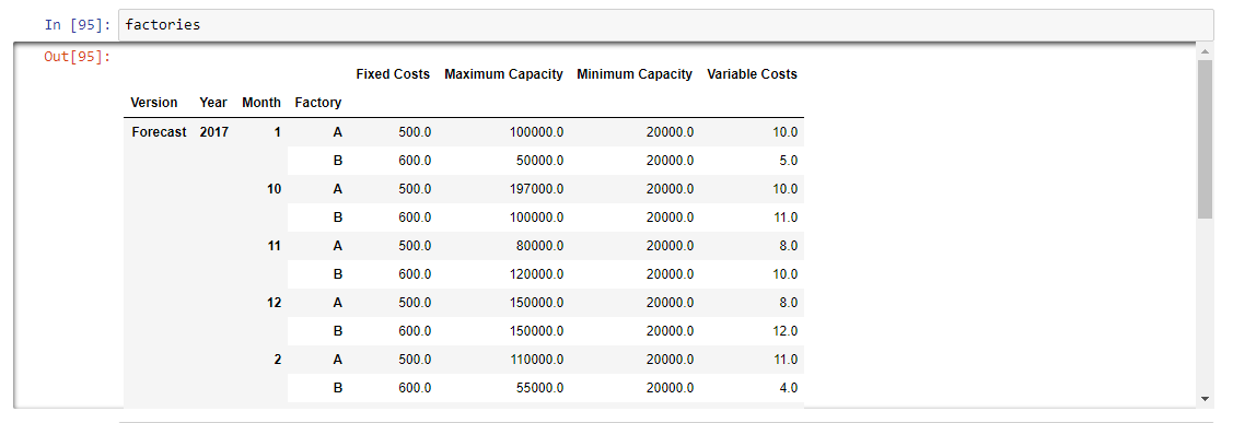
# Reset df index
df = df.reset_index()
index = ['Version', 'Year','Month','Factory','Measure REV Factory Schedule']
df = df.set_index(index)

# Unstack the DataFrame
df = df.unstack(4)
df = df.reset_index()

# Bring TM1 Measures to the same level as dimensions

# Dimensions are stored at level 0
lv0 = df.columns.get_level_values(0)

# Measures are stored at level 1 (in this instance)
lv1 = df.columns.get_level_values(1)

# Collate the columns
columns = lv0[:4]
columns = columns.append(lv1[4:])

# Reset the column values
df.columns = columns

# Set factories index
index = ['Version','Year', 'Month', 'Factory']
factories = df.set_index(index)
factories = factories.fillna(0)
If you display the factories data frame you’ll notice that the data frame measures are now separate columns. This isn’t really all that important from a coding standpoint but it makes it a whole lot easier to interpret. The last line also fills in any blank cells with zero, by default Pandas will set any missing values to ‘NaN’.
2. Install and Import PuLP
Now that that’s out of the way time to get stuck into the actual linear programming. The most intuitive linear programming module for python is PuLP. There are a few other packages out there but this one just seemed to make sense.
Before writing any statements you’ll need to install PuLP. To do this, run the following command using your terminal.
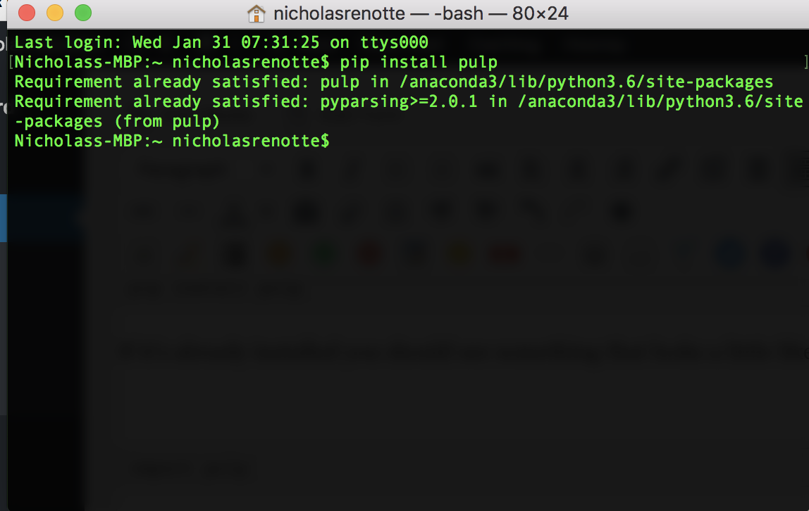
pip install pulp
If it’s already installed you should see something that looks a little like this.
Now that’s out of the way, you’re ready to roll. The first step is to import the PuLP module into the Jupyter notebook.
import pulp
3. Build the Linear Programming Problem
Just like the pizza example at the start of this post, there are different problem components that need to be constructed when using PuLP.
Because this example is to do with optimal scheduling there are two key variables that you’ll want to be calculated. The first one is the level of production aka the number of products each factory should produce.
production = pulp.LpVariable.dicts("production",
                                     ((version, year, month, factory) for version, year, month, factory in factories.index),
                                     lowBound=0,
                                     cat='Integer')
The next variable is factory status. This will hold a binary value, 1 = factory is running or 0 = factory is idle.
factory_status = pulp.LpVariable.dicts("factory_status",
                                     ((version, year, month, factory) for version, year, month, factory in factories.index),
                                     cat='Binary')
The goal of this problem is to produce enough products to meet demand whilst minimising the costs incurred. The next block creates a linear programming problem and sets the target to minimise the target variable, cost. This is done by passing the constant pulp.LpMinimize into the LpProblem method below.
model = pulp.LpProblem("Cost minimising scheduling problem", pulp.LpMinimize)
The cost of production is equal to Variable Costs * Production + Factory Status (i.e. on or off) * Fixed Costs. Using pulp.lpSum we’re able to construct this function for each version, year, month and factory and add it to the model.
model += pulp.lpSum(
    [production[version, year, month, factory] * factories.loc[(version, year, month, factory), 'Variable Costs'] for version, year, month, factory in factories.index]
    + [factory_status[version, year, month, factory] * factories.loc[(version, year, month, factory), 'Fixed Costs'] for version, year, month, factory in factories.index]
)
4. Set Problem Constraints and Solve
So far, the model contains the production and factory status variables as well as the problem objective and the function to minimize. Up until now, we haven’t actually set any constraints on the model.
Constraint 1: Production needs to meet demand
The company is going to have an issue if manufacturing is unable to meet demand. They don’t really care how this achieved as long as the combined production from factory A and B meets the total demand level for the month.
for version, year, month, measure in demand.index:
    model += production[(version, year, month, 'A')] + production[(version, year, month, 'B')] == demand.loc[version, year, month, measure]
Constraint 2: Production needs to be within Max and Min capacity or zero (factory is off)
# Production in any month must be between minimum and maximum capacity, or zero.
for version, year, month, factory in factories.index:
    min_production = factories.loc[(version, year, month, factory), 'Minimum Capacity']
    max_production = factories.loc[(version, year, month, factory), 'Maximum Capacity']
    model += production[(version, year, month, factory)] >= min_production * factory_status[version, year, month, factory]
    model += production[(version, year, month, factory)] <= max_production * factory_status[version, year,month, factory]
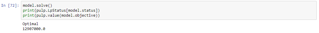
Now there’s nothing left to do but to solve the problem and get the results. Running model.solve simultaneously solves the problem. The two lines below output the model status and the lowest expected cost that will meet demand.
model.solve()
print(pulp.LpStatus[model.status])
print(pulp.value(model.objective))
The model status tells you whether or not the problem was able to be solved. If a suitable solution was found then the status will be Optimal. If not the model will return a status of Not Solved, Infeasible, Unbounded or Undefined.
5. Collate Results and Send to TM1
The final step is to send the results back into TM1. The two values that need to be sent back into the cubes are the production level and factory status indicator. These values are stored in two dictionaries called production and factory status from the previous modeling steps. We can loop through these and add the measures required to send the values back into TM1. To make it clearer, the new values are stored in two separate dictionaries called production_output_cellset and factory_status_cellset.
production_output_cellset = {}
factory_status_cellset = {}
for version, year, month, factory in production:
    production_output_cellset[(version, year, month, factory, "Production Output")] = production[(version, year, month, factory)].varValue
    factory_status_cellset[(version, year, month, factory, "Factory Status")] = factory_status[(version, year, month, factory)].varValue
Then send the values back into the REV Factory Schedule cube using the write_values method.
# Create new instance of TM1 Service object and load data
with TM1Service(address= address, port=port, user=user, password=password, ssl=ssl) as tm1:
   tm1.cubes.cells.write_values('REV Factory Schedule', factory_status_cellset)
   tm1.cubes.cells.write_values('REV Factory Schedule', production_output_cellset)
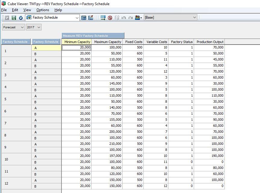
You should ideally see something that looks a little like what’s below in TM1. But wait, I know what you’re thinking…there’s no cost figures here…..
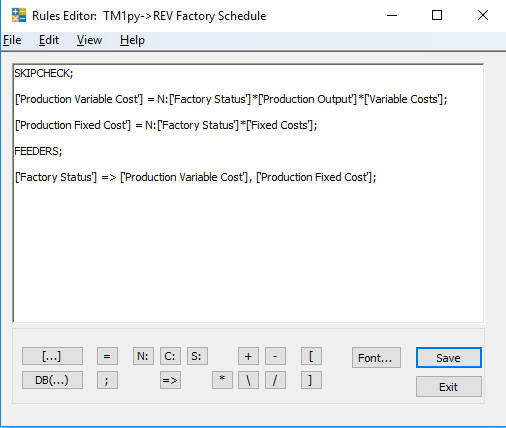
Add the following rule to the Factory Schedule cube to calculate Fixed and Variable costs.
SKIPCHECK;

['Production Variable Cost'] = N:['Factory Status']*['Production Output']*['Variable Costs'];

['Production Fixed Cost'] = N:['Factory Status']*['Fixed Costs'];

FEEDERS;

['Factory Status'] => ['Production Variable Cost'], ['Production Fixed Cost'];
It should look a little like this.
Voila, you now have the optimal level of production and factory status within the cube. Note that the Total Production Cost for all factories matches the optimal figure that was calculated when the model was solved.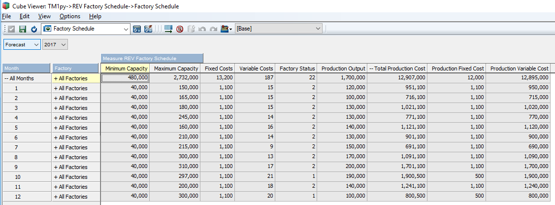
And that’s it. You now have a complete model to calculate optimal scheduling. If you haven’t done so already, download the code and get it up and running! Also, If you want to get a better idea of how to write problems and solve them using PuLP I highly recommend checking out checking out the series over at Ben Alex Keen’s data science blog.